5.9.1. Introduction

5.9.1.1. Basic GUI Appearance

The basic GUI appearance of Gravis is shown in Figure The basic GUI appearance of Gravis.

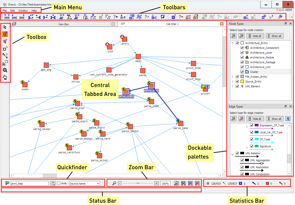
The basic GUI appearance of Gravis

Some elements of the UI can be placed and reordered dynamically. The default arrangement is:

• The main menu at the top.

• Toolbars under the main menu containing certain menu items for quick access.

• The central tabbed area containing the View Box, graph windows, and additional information windows. After an RFG has been loaded, the initial tab in the area is the View Box which

  • contains a list of the views of the RFG;

  • allows opening new graph windows;

  • closes the entire RFG when closed.

• The Toolbox on the left. The Toolbox grants access to the available tools for the current graph window. Its contents depends on the type of window that is active.

• Dockable palette windows on the right. Their contents may change depending on the active graph window. The Node Types and Edge Types palette windows display the scheme of the graph, i. e., the available node and edge types. They are also used to select which type to use for newly created nodes and edges, and they contain checkboxes to control the visibility of nodes and edges based on their types (dynamic filtering by type).

• The Quickfinder (see section The Quickfinder), the Zoom Bar (see section Zooming and Scrolling) and the Statistics Bar (see section The Statistics Bar) below the central tabbed area.

• The status bar at the bottom. It displays help and status information.

There can only be one View Box tab in the central tabbed area. As soon as the View Box is closed, all other windows in that area are closed as well.

Managing your tabs

You can close all open tabs (apart from the View Box) by opening the context menu over one of the tabs and choosing Close all tabs. Choosing Close all tabs but this instead leaves the tab open over which the context menu was opened. Close tabs to left and Close tabs to right close all tabs to the left or right of the current tab, again without closing the View Box.

5.9.1.2. Graph Files

The main menu entry File → Open... opens an RFG or GXL file as a new graph. Alternatively, File → New graph... creates a new empty graph. If there was already a graph loaded, it is replaced by the newly created/loaded graph.

After a graph has been created or loaded, the View Box appears (see Section View Box) displaying a list of its views, and the Node Types and Edge Types palettes display the graph’s schema, i. e., its available node and edge types.

The graph’s attributes can be viewed and edited via Edit → Graph properties.... This opens the Graph information window displaying a list of attributes. Section Editing Attributes explains how attributes are edited.

5.9.1.3. Graph Elements: Nodes and Edges

In the buttons and menu items shown in the Gravis UI, nodes and edges are depicted by the icons and respectively.

In a graphical window, the type of a node is indicated by the shape and color of its graphical symbol. Edges are shown as arrows between node symbols. The type of an edge is indicated by its color, its dash pattern, and the shape of its arrow head . Gravis comes with a default color scheme for nodes and edges. This scheme can be adapted via the Gravis configuration.

Nodes and edges can display textual labels. By default, each node displays the contents of its Source.Name attribute underneath its symbol. This can be adapted and extended via the Gravis configuration, see Section Visualization options.

Note

An overview of the graph element types used in an RFG representing a software system under analysis is given in Language Schema.

The Node Types and Edge Types palette windows contain a list of available node and edge types respectively. These palette windows also serve as a filter facility in graph windows and for choosing the type of new graph elements for the Node Tool and Edge Tool.

5.9.1.4. Views

A view is a subgraph of the RFG. A view captures one particular aspect of the software under analysis (e. g. a call graph, a file and directory hierarchy, an include graph etc.).

A view is depicted by the icon in the UI of Gravis.

Figure Example of nodes and edges in multiple views. shows three views which contain different subsets of the same nodes and edges.

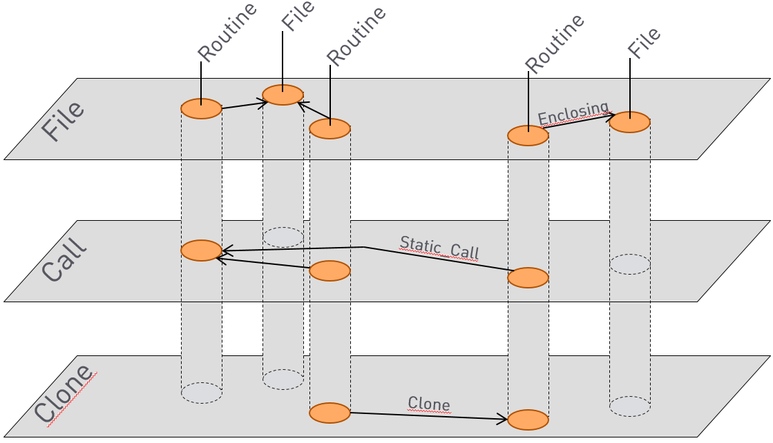
Example of nodes and edges in multiple views.

Caution

Most editing operations in Gravis graph windows (see Section Windows) act on the view the window represents (shown in the window’s tab), so if you choose to delete an element, it is only deleted from this particular view and may remain present in other views. An element is completely removed from the RFG after deleting it from all the views it appears in.

View Box

The View Box (see Figure The Gravis View Box.) represents the graph as a whole and shows a list of all views, their assigned roles (in the leftmost column) and statistics (the number of all/selected/marked nodes/edges in each view).

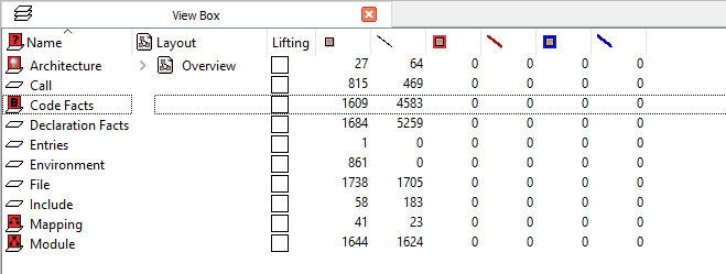
The Gravis View Box.

Double clicking a view without assigned role ( ) in the View Box or choosing Open → Hierarchical... from the view’s context menu opens a hierarchical graph window for that view. The root nodes of the hierarchy in the view will be displayed in the opened window.

The context menu of the View Box additionally allows opening a view

• as a tree window by choosing Open → Tree...

• and as a flat graph window that does not interpret the hierarchical edges by choosing Open → Flat....

Double clicking a view with role Mapping opens a mapping window (see Section Mapping Window).

Double clicking a view with any other role opens a hierarchical graph window for that view (see Section Graphical Windows).

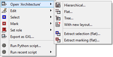
The Open submenu of the View Box context menu.

Creating and Editing Views

A new (empty) view is created using New view from the main menu. This opens a dialog in which the view name can be entered.

Caution

The maximum number of views in an RFG is limited to 64.

Edit → View properties... opens the View information window, in which the view’s attributes can be inspected and edited (see Section Editing Attributes).

A view is renamed using Edit → Rename view... and deleted using Edit → Delete view from its context menu in the View Box.

Edit → Delete Selection and Edit → Delete Marking are short-cut operations allowing you to delete the selected/marked elements in the given view without having to open a graph window first.

View Operations

Views can be manipulated as a whole. To copy a view, use Edit → Copy view... and enter a name for the copy. The Union, Intersection, Difference, and Symmetric difference operations combine two views, so the second view needs to be chosen from the item’s submenu.

Copying Elements Between Views

Edit → Copy selection to and Edit → Copy strict selection to copy the selected elements in the view to the view chosen from the submenu. The difference between the two operations is only in the handling of selected edges whose attached nodes are not both selected as well. Copy selection to always includes selected edges, copying their attached nodes as well, no matter whether they are selected or not. Copy strict selection to excludes selected edges that are attached to unselected nodes.

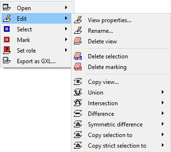
The Edit submenu of the View Box context menu.

View Roles

The role of a view defines the meaning of that view in the context of certain analysis or editing steps, most notably, architecture analysis (see Section Architecture Analysis Facilities). Each view can have at most one role, and each role can only be assumed by a single view. The role of each view is depicted as a red icon to the left of its name in the View Box. It is set using Set role in the View Box context menu.

Exporting and Importing Views

Views can be exported as separate GXL files. The GXL format is an XML-based format that captures one or more views of an RFG.

Note

Manually created views like architecture and mapping views must be kept separate from the source analysis result. This allows these views to be shared by several versions or variants of the software system under analysis.

The context menu in the View Box contains Export as GXL... for exporting a single view or a selection of views as a GXL file. The main menu contains the item File → Import views... for importing views. It allows you to select one ore more GXL files and imports them into the graph. File → Import recent leads to a submenu of recently imported view files for quick access.

Note

If architecture and mapping are modeled using Gravis, the RFG obtained from the dashboard might already contain the architecture and the mapping (depending on the configuration of the analysis process).

Caution

The identity of graph elements is managed by their attributes and types, most notably the Linkage.Name attribute is used to identify nodes. When importing a GXL file into an RFG, nodes with matching names are shared between the existing views of the RFG and the imported view(s), whereas any nodes that were not found in the RFG are imported as new nodes. If any node names were changed in the RFG between exporting a view and re-importing it, the names may no longer match.

5.9.1.5. Layouts

Gravis keeps the core graph model (nodes, edges, views and their attributes) and layout information strictly separate, because in a typical environment with continuous integration, there are regular automated analysis runs that produce updated versions of the RFG from the current state of the analyzed software system. If the layout information was part of the RFG file, it would be overwritten when replacing the RFG by an updated version.

Transient layouts

By default, when you double-click on a view to open it in a graph window, it is opened with a transient layout. That means that the nodes get some automatic initial positions (e. g., they are arranged in a regular grid) and any changes you make to the layout, e.g., by moving, expanding and resizing nodes, are discarded when you close the window. The next time you open the same view, it is displayed with an automatic layout again. While this is sensible behavior for inspecting views, e.g., the Code Facts or Call views, this is not helpful when modeling a view, e. g., an architecture. When doing that, node positions and sizes should be remembered.

You can save the current layout of a graph window to a file at any time, allowing you to restore your layout the next time you open the same view by reloading the saved file. In principle that would allow you to manage your layouts, but this manual process is cumbersome and error prone. For instance, after having rearranged some nodes, it is all too easy to forget to save the changed layout before closing the graph window.

Persistent layouts

Gravis offers named persistent layouts that are associated with a particular view in a particular RFG. If a view is opened with a persistent layout, then the graph window “remembers” which layout it edits and asks you whether you want to save any changes when you close it. At any time, while editing a persistent layout, you can update the saved layout easily, revert to the last saved state or even create a new persistent layout with a different name from the current layout shown in the window. You can create any number of persistent layouts for each view of a graph. One of these layouts has the special role of being the default layout. This layout is used when you double-click on the view in the View Box.

Layout management in the View Box

To create a new persistent layout for a view, choose Open → With new layout... from the context menu over a view entry. This creates a new layout and immediately opens a window with a hierarchical display. If the new layout is the first layout created for the view, it automatically becomes the default layout.

The View Box shows the default layout of each view in the “Layout” column. An arrow (>) in front of the default layout name indicates that there are additional layouts for the view. Clicking on the arrow expands the list of additional layouts. Clicking again collapses the list.

Double-clicking on any row with a layout opens the view with the given layout. It is still possible to open a view without using any of its available persistent layouts (i. e., with a transient layout) by choosing Open → Open flat... or Open → Open hierarchical... from the context menu over a view entry.

Note

Using Open → With new layout... always creates a hierarchical layout. If you want to create a flat persistent layout, choose Open → Open flat... and then create a layout using Layout storage → Create new layout... in the context menu of the graph window.

The context menu over a layout item shows additional options at the top of the menu:

• Open ’<layout name>’... is equivalent to double-clicking: It opens the view with the given layout.

• Rename layout... opens a dialog box in which you can enter a new name for the layout.

• Delete layout... deletes the layout.

• Make default layout makes the clicked layout the default layout and moves it next to the view name. The former default layout takes the place of the clicked layout.

• Copy layout to allows you to choose the target view from a submenu and copies the clicked layout to the target view. This only makes sense if the target view contains roughly the same nodes as the view from which the layout is copied (or a superset of the nodes). One example where this is useful is to copy layouts from an architecture view to the result view of an architecture analysis run.

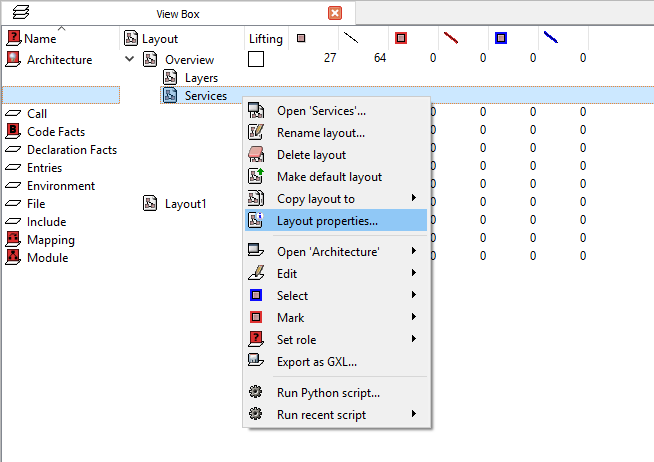
The context menu over a layout entry in the Gravis View Box.

Working with persistent layouts

Double-clicking on a view with a persistent layout in the View Box (or using Open ’<layout name>’... from the context menu over a layout) opens a window showing the view with the chosen layout. The window’s tab displays the name of the edited layout. Each layout can only be opened once, so double-clicking on the same layout a second time simply activates the tab with the open graph window instead of opening a new window.

Any changes to the layout (node positions and sizes, expansion state, hidden nodes and edges, etc.) are persistent, i.e., they are saved when the window is closed or when Gravis is quit. The saved state also includes the zoom factor, the area of the graph shown in the window, the visualization options and the hidden node/edge types.

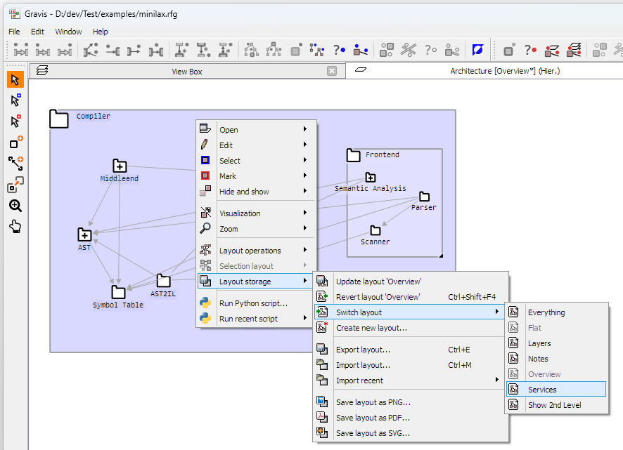
The context menu over a graph window with a persistent layout.

While editing with a persistent layout you can update the saved state of the layout by choosing Layout storage → Update layout ’<layout name>’ or revert the displayed layout to the most recently saved state by choosing Layout storage → Revert layout ’<layout name>’ from the context menu over the graph window. You can switch to a different layout by choosing it from the submenu of Layout storage → Switch layout. If the current layout is modified, you are prompted to save your changes first.

You can create a new persistent layout based on the current state of the window by choosing Layout storage → Create new layout.... This opens a window in which you can enter the name for the new layout. The new layout then becomes the one that is currently edited in the window.

Create new layout... is available in windows editing a transient layout, too. You can also switch from a transient layout to a persistent layout by choosing a layout from the Layout storage → Apply layout submenu.

If you close a window with a modified persistent layout, Gravis asks whether is should be saved. This query can become annoying, so you can tick Always save layouts without asking to stop it from appearing in the future. This setting remains active for the current Gravis session.

Automatic creation of persistent layouts

Views can be marked to use persistent layouts automatically. When creating a view via New view, ticking the option Use persistent layouts sets a view attribute indicating that this view should preferably be opened with a persistent layout. The attribute name is Gravis.Persistent_Layouts, and it can be set manually via the View properties... dialog, too. After creating a view with this attribute, or when importing such a view from a .gxl file, Gravis automatically creates a persistent layout for it. That avoids accidentally opening the view with a transient layout. It is recommended to tick this option when creating a view for modeling a system architecture.

Persistent layout storage

By default, persistent layouts are stored in a directory alongside the RFG file with the same base name as the RFG file, but with the .rfg extension replaced by .gls (“Gravis layout storage”). If your RFG files are usually stored in a read-only location, you can force Gravis to store all persistent layouts in a separate directory by setting the configuration option /Tools/Gravis/layout_directory to an existing writable directory.

Pending layouts

When a view is deleted, any layouts associated with the view can be kept as “pending” layouts. These are not shown in the View Box, but remain in the layout directory, ready to be reused. If a view with the same name is subsequently created or imported, the layouts are reactivated automatically and shown alongside the view.

Pending layouts are useful when replacing an architecture view that was imported from an external source (e. g., a third-party CASE tool) with a later version. This is usually done by first deleting the Architecture view from the graph and then re-importing a new .gxl file created by the importer. If the Architecture view has any persistent layouts when it is deleted, then Gravis asks you whether these layouts should be kept. After clicking on Keep layouts to keep them and re-importing the updated Architecture view file, the newly imported view still has the layouts of the original view.

Note

Pending layouts are only reactivated when creating or importing a view with a name for which pending layouts were previously kept. When an existing view is renamed, it always retains its existing layouts, even if there are any pending layouts for the new view name. Such pending layouts are deleted.

When closing the graph or quitting Gravis, there may still be pending layouts around. These could be layouts that you chose to keep when deleting views, or layouts referring to views that you created in the graph but subsequently discarded by choosing not to save the graph. In either case, Gravis offers you to delete these layouts, because their presence might surprise you in the future when creating/importing a view with a matching name.

Layouts and screen pixel densities

Starting from version 7.6.8 Gravis supports moving layouts between systems with different pixel densities (and therefore different system DPI scaling). For instance, that allows the same layout files to be used on a system with a conventional full HD display and a system with a 4k display. Previously, layouts saved on a standard density screen would be shown at half the size on a 4k display. Now, the layout contains information about the DPI scaling that was in use on the system on which the file was saved, so all pixel sizes in the file can be rescaled correctly on a target system with a different DPI scaling setting.

Values that are affected are:

• Node symbol sizes

• Node positions

• Expanded node sizes

This only works as expected if the layout was saved on at least version 7.6.8, so any older layouts need to be resaved to become interoperable. For layouts saved using Layout storage → Export layout..., this means importing the layout and re-exporting it. For persistent layouts (see Working with persistent layouts), this means opening the view with the given layout, making a tiny change like moving a node slightly to make Gravis consider the layout to be modified and then choosing Layout storage → Update layout ’<layout name>’.

Starting from version 7.12, Gravis also supports moving graph style configurations between systems with different pixel densities because all measurements in the configuration are now interpreted as device-independent pixels that are scaled by the system DPI scale factor.

5.9.1.6. Toolbox and Cursors

Depending on the type of the currently active graph window, the Toolbox contains a selection of these tools:

Icon	Tool	Shortcut	Cursor	Purpose
				continued on next page
	Navigate	F3		Expand, resize, and move elements
	Select	F4		Select and move elements
	Mark	F5		Mark and move elements
	Node	F6		Create nodes
	Edge	F7		Create edges
	Hierarchy	F8		Edit node hierarchy
	Zoom	F9		Zoom in/out
	Scroll	F10		Scroll the canvas
	Map	F11		Edit architectural mapping

The currently selected tool determines what happens when you click into a graph window. For instance, the Select Tool selects a clicked graph element and the Node Tool creates a node at the click position. Some tools also support drag operations on graph elements or on the window background: For instance, the Select Tool allows you to move nodes by dragging them, but also to drag a box on the window background around several graph elements to select them in one go. The Zoom Tool allows you to zoom to a particular area of the window by dragging a box around it.

The cursor shape changes according to the selected tool, the element under the cursor and the action that is in progress. For instance, while the cursor points to an edge, the Navigate, Select, and Mark cursors show an additional edge symbol. That makes it easier to “hit” an edge, e. g., in order to select it or to open its context menu. If the element under the cursor can be moved, the cursor changes to a four-headed arrow.

The keyboard shortcuts for the tools shown above are the defaults. See Keyboard shortcuts for customization options.

5.9.1.7. Gravis Scripting

Gravis can be extended using Python scripts. Scripts can inspect and manipulate the loaded RFG, change the selection and marking, open new windows and even traverse and manipulate the graphical representations of RFG elements. Python scripts can be launched via File → Run Python script... on the main menu or from the same entry on the context menu of the View Box, graph and edge list windows. Scripts launched from the View Box have access to the view over which the context menu was opened and to the selected views. Scripts launched from a graph window have access to the graph element over which the context menu was opened. The details of Gravis scripting are described in the Gravis Scripting Guide.

Scripts can be added to menus and be given keyboard short-cuts, so they appear in the user interface like native Gravis features. You can also add scripts that are run automatically in specific situations, e.g., after a node or an edge has been created. See Section Adding Scripts to Menus, Shortcuts and Events.

5.9.1.8. Configuration

Like the other tools of the Axivion Suite, Gravis reads its configuration by consulting the BAUHAUS_CONFIG environment variable, but in addition to that, it also reads an optional extra configuration file gravis.json in the .bauhaus directory inside the user’s home directory (see User-specific settings).