
5.9.2. Windows
The elements of a view can be visualized in graph windows. Graph windows can show a graphical representation of the nodes and edges in a view or a tree representation of just the node hierarchy. It is possible to open several windows for the same view.
Graphical windows can be flat or hierarchical. A flat window has no special treatment for hierarchical edges and displays them as ordinary edges between nodes. A hierarchical window interprets these edges as an indication of hierarchical nesting, i. e., they indicate which nodes are inside or part of a parent node. Tree windows are always hierarchical.
Operations that take the hierarchical structure of nodes into account are sometimes called “deep operations”.
5.9.2.1. Graphical Windows
Graphical windows are opened by double-clicking on a view entry in the View
Box or by choosing

Open → 
Flat... or
Open → 
Hierarchical...
from the context menu over a view entry.
Hierarchical Navigation
When a flat graph window is first opened it shows all nodes and edges in the view at the same time, even hierarchical edges. This allows the hierarchy to be visualized as a graphical tree structure.
In contrast, when a hierarchical graph window is first opened, only the root nodes of the view are displayed. A small plus sign inside a node icon indicates that the node has children and that it can be expanded to reveal its contents.
Expanding and Collapsing Nodes
In the 
Navigate, 
Select,

Mark, 
Node Tool or 
Hierarchy Tool, double clicking on a closed node expands it and displays
its direct children in its expanded node area. In addition to the edges between child
nodes, this also reveals edges between any of the child nodes and other nodes located
outside the expanded node.
Double clicking an expanded node collapses it again, i. e., removes its expanded area including its children from the display. Consequently, edges from other nodes to child nodes become invisible, too.
See Figure Before and after expanding node “Compiler” for the effect of expanding a node
in the Architecture view of an example.
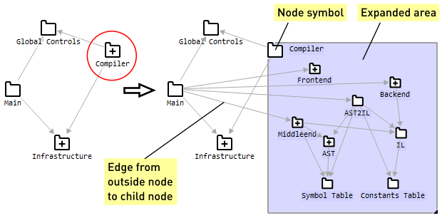
Before and after expanding node “Compiler”
You can expand or collapse multiple nodes in one go using the

Expand selected nodes,

Collapse selected nodes,

Expand marked nodes, and

Collapse marked nodes operations in the

Visualization sub-menu.
Locating Nodes in the Hierarchy
In a deeply nested hierarchical structure it can be difficult to find a particular node
or set of nodes. After selecting or marking nodes
(see Section Working with Selections and the Marking),
Visualization → 
Expand
to show selected or 
Expand to show marked
expands the required levels until all selected/marked nodes are displayed.
Note
In order to locate a node with a particular name in a hierarchical graph or tree
display, you can select it using the Quickfinder
(see Section The Quickfinder) and then use
Visualization → Expand
to show selected. In order to select nodes or edges based on more complex
conditions, use the

Select → 
Select
by query... operation (see Section Query-based operations).
The Expanded Node Area
The expanded area of a node can be resized by dragging the handle in its bottom right corner. It is not possible to make the area smaller than the area occupied by its child nodes (including some minimal margin). However, it is possible to scale the positions of children in the area by Ctrl dragging the handle. This operation places the children at the relative positions they had before the drag.
Double clicking the handle minimizes the area of the node to the space it needs to
encompass all its children. The same can be achieved using
Visualization → Shrink node
to fit from the context menu. Holding down Shift while double clicking the
handle shrinks all children recursively first (
Visualization → Shrink to fit
(deep) from the context menu).
In most tools (e. g., Navigate, Select and Mark), it is not possible to move a child node outside the node area of its containing parent node. Moving a child to the right or below the bottom edge enlarges the parent area to encompass the node in its new position. Moving it to the left or above the top edge is not possible.
Note
You can only drag nodes out of their parent containers into other containers using
the Hierarchy Tool
(see Section Editing the Hierarchy), which allows you to edit the
hierarchical structure of nodes.
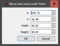
Expanded area size
The context menu entry Visualization →

Position and size... opens a dialog that allows you to
set the position and size of the node numerically. The size can only be set for expanded
nodes. The position is measured in absolute pixel coordinates for top-level nodes. For
nodes that are nested inside other nodes, it is the relative position inside the parent
node’s expanded area, with the parent node being at position (0, 0). The positive
horizontal axis points to the right, the positive vertical axis points downwards.
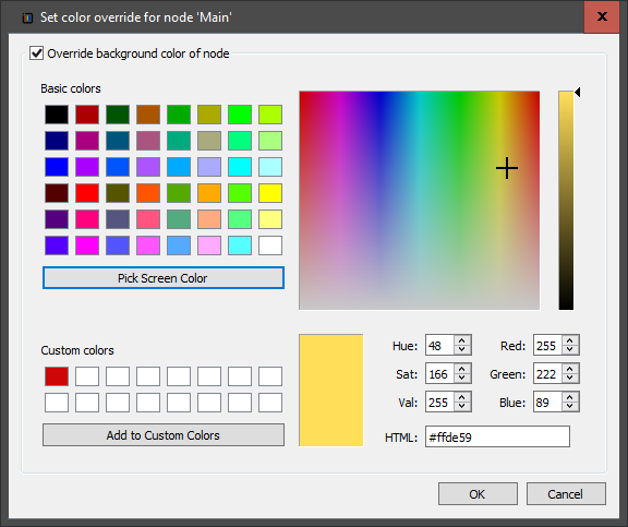
Expanded area color
The context menu entry Visualization →

Node color... opens a dialog that allows you to override
the expanded background color of the clicked node. By default, this color is defined
by the configured style for the node’s type. To override it, enable the option
Override background color of node at the top of the dialog and choose a
color from the color picker. To reset the node to its original color, disable the
option at the top of the dialog.
Note
The color override becomes part of the layout and is stored in saved layout files.
Avoiding Overlapping Node Areas
By default, expanding a node does not move other nodes out of the way, so in particular
after using Expand to show selected/marked many nodes might be hidden
under the expanded areas of opened nodes, or even the expanded areas themselves might
overlap.
Overlaps can be eliminated using
Visualization → 
Remove
overlaps, which moves the nodes at one level around to avoid any overlaps.
Visualization → 
Remove
overlaps (deep) does the some for an entire nested hierarchy, i. e., it recursively
removes overlaps in expanded child areas before doing the same at the parent level.
In the Navigator Tool, a double click inside an expanded area of a
node or at the top level does the same as “Remove overlaps”. Shift double
clicking does the same for the whole hierarchy (“Remove overlaps (deep)”).
Note
Shift double clicking at the top level (i. e., on the window background) removes all overlaps in the entire graph window.
The visual behavior of overlapping nodes are influenced by the
Visualization settings in the context menu of the graph window, in
particular the Semi-transparent backgrounds option, which controls whether
expanded node backgrounds are fully opaque or semi-transparent.
Summary Edges (“Lifting”)
While a node is collapsed, there is no indication that there are edges from the outside to one or more of its children, as can be seen on the left hand side of Figure Before and after expanding node “Compiler” on page . To give a better impression of the graph structure, views can be enhanced with summary edges that are shown between collapsed nodes to indicate that there are edges between their children (or even more deeply nested descendants). Views with these extra summary edges are called “lifted” views, and the summary edges are called “lifted” edges.
Gravis can show any view with lifted edges. This is controlled using the checkbox
icons in the Lifting column in the 
View Box. If the
checkbox is in state “off” (  ), there are no lifted edges. Enabling the
checkbox causes lifted edges to be added to the view. The checkbox shows a tick to
indicate that the view contains lifted edges. By default, the lifting is updated
automatically if the view is edited. This is indicated by a green “update” icon next to
the tick (
), there are no lifted edges. Enabling the
checkbox causes lifted edges to be added to the view. The checkbox shows a tick to
indicate that the view contains lifted edges. By default, the lifting is updated
automatically if the view is edited. This is indicated by a green “update” icon next to
the tick (  ). Automatic updates can be slow in views with many nodes
and edges, so you can switch from automatic to manual updates by clicking on the
checkbox again. The icon changes to an ordinary tick (
). Automatic updates can be slow in views with many nodes
and edges, so you can switch from automatic to manual updates by clicking on the
checkbox again. The icon changes to an ordinary tick (  ) to indicate
that the lifted edges are no longer updated automatically. Clicking on the checkbox once
again causes the lifted edges to be deleted and removed from all open diagrams showing
that view. The checkbox returns to its original state ( ).
) to indicate
that the lifted edges are no longer updated automatically. Clicking on the checkbox once
again causes the lifted edges to be deleted and removed from all open diagrams showing
that view. The checkbox returns to its original state ( ).
If automatic updates are disabled and the view is edited in a way that invalidates the
lifted edges (e. g., if edges are deleted or nodes are moved within the hierarchy), the
checkbox displays an “outdated” marker next to the tick (  ).
Clicking on the marker updates the lifting, and the icon changes back to an ordinary
tick ( ).
).
Clicking on the marker updates the lifting, and the icon changes back to an ordinary
tick ( ).
Alternatively, you can switch between the different states by choosing an option from
the context menu over the Lifting column. It offers
Add lifted edges and

Delete lifted edges to switch lifting on and off,

Update lifting to update lifting that has become
outdated and Auto-update lifting to switch between manual
and automatic updates.
Caution
The lifted edges shown via this method are not really part of the graph, so they
cannot be selected, marked or deleted, and they are not saved to .rfg or
.gxl files.
Note
It is also possible to create a lifted version of any view using the
Lift edges totally operation available in the Analysis Window (
Edit → 
Run Analysis... from the
main menu). In contrast to dynamic lifting using the lifting icon in the
View Box, this operation creates static edges, i. e., real edges
that can be selected and deleted and that become part of the .rfg or
.gxl file if the graph is saved.
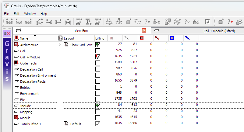
Various lifting states shown in the View Box
In Figure Various lifting states shown in the View Box, the view “Architecture” has
automatically updated lifting, “Call + Module” and “Include” have manually updated
lifting, and that of “Call + Module” is out of date. Finally, “Totally lifted 1” has
statically lifted edges created by the Lift edges totally operation - the
tick indicates that there are lifted edges, but the button is grayed out, since the
lifting state cannot be changed. The other views are not lifted.
Working with lifted views
Double-clicking on a lifted edge (no matter whether it was created by dynamic or static lifting) displays an edge list window (see Section Edge List Windows) containing the real edges that were represented by the lifted edge.
In a window showing a lifted view, the display of summary edges can be switched off by
unticking
Visualization → Show lifted
edges.
Architecture analysis creates dynamically lifted edges for its result edges and for the source code edges that caused architecture violations, see Section Interpreting the Result of Architecture Analysis. Lifted architecture analysis result edges behave more intelligently when double clicked: Instead of showing the real result edges represented by the lifted result edge, the opened edge list window shows all the causing edges responsible for the result edges, grouped by result edge. See Section The graphical Architecture Check result view.
Common Operations in Flat and Hierarchical Windows
Layout of Nodes
The layout of nodes can be changed
by manually dragging the node icons while the
Navigate, Select, Mark, or Hierarchy Toolis active,by applying a layout operation from the

Layout operationssubmenu to lay out all nodes in the area over which the context menu has been openedby applying a layout operation from the

Selection
layout
submenu to lay out just the selected nodes in the area over which the context menu has been opened
Opening the context menu on the background of the graph window lays out all top-level nodes. Opening the context menu over an expanded node background lays out the children of that node.
Note
Most Selection Layout operations lay out the
selected nodes in the space (enclosing rectangle) currently occupied by the nodes.
Bringing Nodes to Front
Clicking on a node (or, in a hierarchical window, also in its expanded area) brings the
node (and its ancestors) to the front.
Visualization → 
Put
node to back
in the context menu inside a node area allows to put the node to the
background (behind all other nodes inside the same parent).
Hiding Elements
Elements can be temporarily hidden from a graph window’s visual representation using the
Hide operations from its 
Hide and
show
context menu. They can be made visible again using the Unhide operations.
Hide and
show → 
Unhide all makes all elements visible again
that were hidden using Hide operations.
The check boxes next to the type entries shown in the Edge Types and
Node Types palette windows allow elements to be hidden dynamically based
on their types. This is independent of the individual hiding status of each node, so if
you hide an individual node, then hide the node type and make the node type visible
again, the individually hidden node remains hidden.
Note
The individual hiding status of nodes and edges and the hidden node/edge types are stored in layout files.
Focus on Nodes
In order to improve the visibility of elements of interest it is possible to focus on
a node or a selection of nodes, i.e., make the nodes in question and their environment
temporarily stand out visually from the rest of the graph. Focusing is done by
Visualization → 
Focus
on node
and
Visualization → 
Focus
on selection
. The focused nodes and all directly attached nodes are displayed normally
in full color, all other elements are shown in faded colors to make them less prominent.
The focus operation is stopped by
Visualization → 
Stop
focus
. All faded elements are displayed normally again.
To make it easy to find endpoints of edges, the context menu over an edge offers the
options Visualization → Focus
on source node and
Visualization → Focus on
target node, which focus on the given endpoint of the edge and scroll it into view.
Multiple Edges and Edge Bundling
If there are several edges between a pair of nodes (typically with different edge types), these are shown as parallel edges. That way, each of the edges can be viewed and selected individually. This level of detail is not always required and too many parallel edges can be messy and distracting.
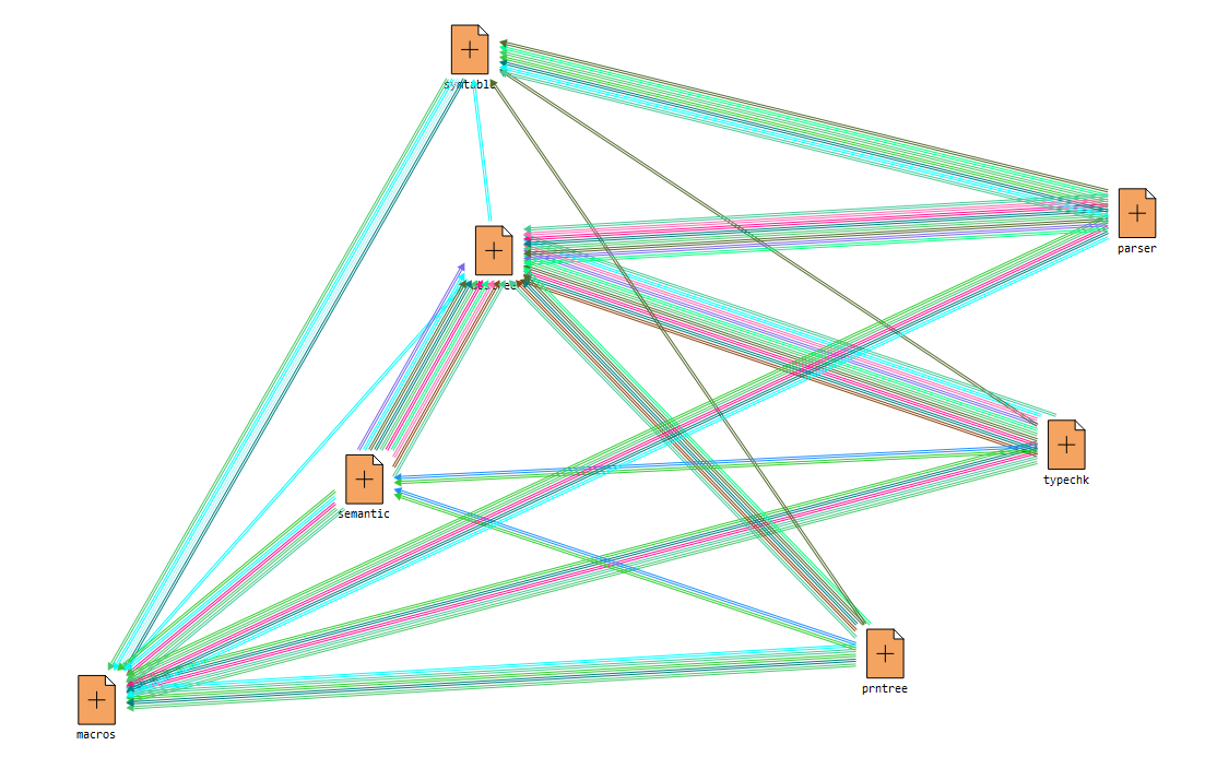
Parallel edges between nodes
Edge bundling replaces all parallel edges
between any given pair of nodes by a single “bundle edge” that represents all the
underlying parallel edges. It is displayed in a more prominent way to make it stand out.
To enable edge bundling, choose Visualization →
Edge bundling... from the context menu. This opens a dialog in which edge
bundling can be enabled/disabled and the bundling threshold can be set. The threshold
is the number of parallel edges starting from which edge bundling happens. If the number
of parallel edges in the same direction between a given pair of nodes is below the
threshold, the edges are shown individually.
You can also press Ctrl+Shift+B to enable/disable edge bundling.
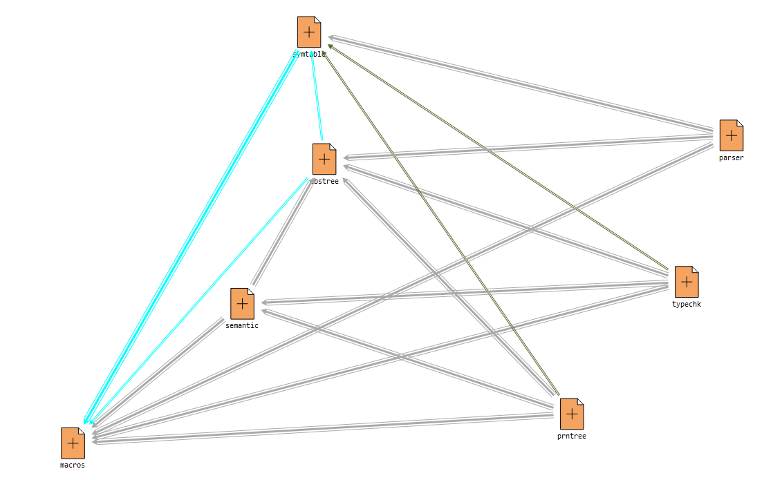
Cleaner display by enabling edge bundling
Each bundle edge is shown using the visualization of the closest common supertype of the
represented edges. For instance, a Set and a Use edge would be
represented by a Reference bundle edge.
Double-clicking on a bundle edge opens an edge list window with the edges that are represented by the bundle.
If some edge types are hidden by filtering (see The Node and Edge Types palettes) then a bundle edge is visible if at least one of the edges it represents is visible.
Saving and Loading Layouts
The current layout of nodes in a graph window can be saved separately from the RFG and
loaded back later. This is done via 
Export layout...
and 
Import layout... in the
Layout storage submenu of the graph window context
menu. Both entries open a file chooser dialog to select which layout file to save/load.
The Import recent entry leads to a submenu with the
most recently exported/imported layout files for quick access.
Layouts are saved as XML files with extension .gvl. A layout file stores node
positions, the expanded sizes of nodes and whether they are collapsed or expanded and
which nodes or edges have been hidden via the operations in the Hide and
show submenu. It also stores the current visualization options and which node and edge
types have been hidden in the Node/Edge Types windows.
Note
The external storage of layouts is especially useful when working with different versions and/or variants of the same system under analysis.
Exporting as PNG, PDF and SVG
The current layout of nodes in a graph window can be exported as a bitmap file in PNG
format by Layout
storage → 
Save layout as PNG..., as a
scalable vector PDF file by Layout
storage → 
Save layout as PDF... and as a
scalable vector SVG file by Layout
storage → 
Save layout as SVG....
Zooming and Scrolling
The 
Zoom Tool allows you to zoom in by clicking into the
graph window, zoom out by holding down Shift while clicking into the graph window
and zoom to a particular area of the window by dragging a box around it. While the
Zoom Tool is selected, the scroll wheel of the mouse zooms in
and out instead of scrolling up and down.
The Zoom Bar at the bottom of the window shows the current zoom factor.
To change it enter a percentage value and press Return or drag the slider to the
left of the field.

The Zoom Bar
The 
Zoom submenu of the context menu offers entries to reset
the zoom factor to 100% (
Zoom to 100%, shortcut
Ctrl + 0), fit the entire graph into the window (
Zoom to graph, shortcut Ctrl + G) and to fit all selected
or marked elements into the window (
Zoom to
selection
and 
Zoom to marking respectively). You can
access these actions from the Zoom Bar as well.
You can zoom in and out in all tools using the scroll wheel by holding down Ctrl.
The 
Scroll Tool allows you to scroll the window contents by
dragging on the window background as a more direct alternative to dragging its scroll
bars.
Adapting the Graph Style
Many aspects of the way in which Gravis displays graphical diagrams can be customized, e.g., colors, node shapes, line widths and labels. See Visualization options.
5.9.2.2. Tree Windows
The tree window shows the hierarchy of nodes in a view as an Explorer-like tree view.
The usual expand/collapse facilities are available, plus
Visualization → Expand
selected nodes, Collapse selected nodes,
Expand marked nodes,
Collapse marked nodes,

Expand all, and 
Collapse all
from the context menu.
The context menu entries
Visualization → Expand
to show selected and Expand to show marked can
be used to locate the selected/marked nodes in the hierarchy.
As in graphical windows, the Select Tool can be used to
select elements by clicking on them. Please note that it is not possible to select a
range of elements by holding down Shift while clicking, which is the usual convention in
a tree view. Instead, Shift clicking has the same meaning as in a graphical view,
i. e., it does deep selection (see Section Selecting Elements).
Instead of holding down Shift , you can select a range of elements in a tree
window by dragging a box around them.
Nodes are sorted alphabetically in the tree view. By default, the name comparison is
case-insensitive, unless you tick
Visualization → Case
sensitive comparison. Ticking
Visualization → Group by
type sorts the elements first by type, then by name within each type group.
Filtering elements
The Filter Box at the top of each tree window allows you to filter the
entries that are shown in the window. Only those entries whose source or linkage names contain
the entered filter string are shown. Pressing Return in the Filter Box expands the whole tree
to reveal all elements.
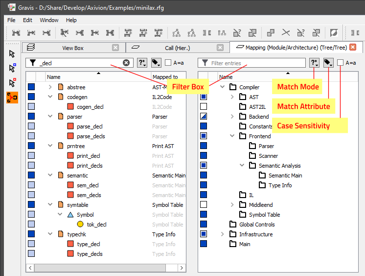
A Mapping Window with Filter Boxes. The left-hand side is filtered.
The three controls next to the Filter Box allow you to fine-tune the filtering:
In the Match Mode control you can choose between standard substring matching
( ), wildcard matching using
 * and + ( ) and regular
expression matching (
) and regular
expression matching ( ).
).
In the Match Attribute control, you can switch between matching the
Source.Name attribute ( ), the
 Linkage.Name attribute
( ), the full file path (
 ) and the
 UML.Stereotypes
attribute ( ). The full file path is the combination of the
 Source.Path
and Source.File attributes. A node with Source.Path = src/module
and Source.File = file.cpp has a full file path of src/module/file.cpp.
Switching the A=a option on makes the match case-insensitive.
Note
In a Mapping Window showing both the architecture and hierarchy views as
trees, each side has its own independent Filter Box.
Caution
Filtering requires Gravis to look at each node in the view, so editing the filter string can be slow for views with many nodes.
5.9.2.3. Subset Windows
A subset window is a flat graph window showing only a certain subset of the nodes in a
view. A subset window can be opened by

Open → 
Extract
selection...
or
Open → 
Extract
marking...
from the context menu of the View Box and of a graph
windows context menu.
Note
Please note that although it is possible to have nodes of different views in the marking at the same time, extracting them into the same subset window is not possible. The opened subset window is always clipped at the view for which it is opened.
Except for the limited number of elements that are shown, a subset window behaves exactly like a flat graph window, so the same operations are available as for a flat graph window.
Even though the subset window only shows a subset of elements of a view, selection
and marking operations still operate on the view, so an operation like
Select → 
Select
incoming edges
may select edges that are not part of the subset.
You can limit the selection to the displayed subset at any time using
Select → 
Clip
selection to visible
.
Alternatively, you can also add these additional nodes and edges to the subset window by
choosing Hide and Show → 
Add selection to diagram. Please note that adding an edge always adds its
source and target nodes to the diagram, too, otherwise the edge would not appear.
Caution
Deletion operations still operate on the view, too, so

Edit → 
Delete and
Edit → 
Delete
selection
not only remove the clicked element/the selection from the subset window
but from the whole view, so they also disappear in other windows showing the same view.
You can remove nodes and edges from the subset window by choosing
Hide and Show → 
Remove
selection from diagram
. Please note that this will always keep the subset in a
consistent state, so removing a node removes its attached edges from the subset, too.
5.9.2.4. Edge List Windows
An edge list window shows a list of edges in a view, typically a subset. Edge list windows are opened by double-clicking on a lifted edge, an architecture result edge or a bundle edge.
Each row of an edge list window represents an edge. You can select, mark, edit and
delete these edges. The nodes that are shown in the Source/Target node columns are
purely for information and are not effected by any operations. If an edge is selected
and/or marked, its row background changes to indicate this. Clicking on a row using the
Select Tool or the Mark Tool
selects/marks the shown edge. Please note that the selection/marking status of the
source and target nodes is not visualized in the edge list window.
Caution
Deleting an edge in an edge list window, deletes it from the view, not just from the window. This is consistent with the behavior in any other window showing graph elements, e. g., graphical windows and tree windows.
5.9.2.5. Source Code Windows
Graph elements originating from source code analysis (e. g., the nodes and edges
in the Code Facts view) are associated with source code positions. You can display a
Source Code window indicating the source location of an element using
Open → 
Show
source code...
from the element’s context menu. The element’s associated source line is
highlighted with a yellow background.
You can zoom into/out of the window by holding down Ctrl and using the vertical mouse wheel.
Apart from displaying the source code, the Source Code window allows code
to be selected by dragging over it using the mouse and copied using Copy
on the context menu or by pressing Ctrl+C.
To find a string in the source code window, use Find... on the context
menu (or press Ctrl+F). This opens the search bar at the bottom of the Source Code
window. Enter the search string into the input field and press Return to search forward
or Shift+Return to search backward. If the option a=A is ticked, the
search is case insensitive, else it is case sensitive. The up/down arrows next to the
input field allow you to search forward/backward using the mouse. The close icon next to
the arrows closes the search bar.
Resolving Relative Source Code Paths
Graph elements often contain relative file paths. These are resolved by prefixing them
with the source base path, which is stored as a graph attribute. If the source base
path is not set up in the graph or if it is incorrect, it can be overridden with a
user-defined source base path in Gravis, either via the command-line option
--basepath <path> when starting Gravis or via the base path dialog (
File → Source base path...). The dialog shows the
source base path stored in the graph and allows you to switch to a user-defined base
path. You can either enter the base path manually or click on Browse...,
which opens a standard file dialog to select the basepath directory.
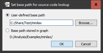
The Base Path Dialog.
Clone Pair Windows
A Clone Pair window is a special type of Source Code window
that displays two source files side by side to compare identical or similar regions of
code found in different source files or in different places within the same file. It is
opened by double-clicking on a 
Clone edge, typically found in
a Clones view, or by clicking on the Show clone pair... button
in the Edge Information window of a clone edge. Each of the two sides
offers the same facilities as an ordinary Source Code window.
External Code Viewers
Gravis can optionally launch an external editor to display source code instead of
using its own Source Code window. You can control this behavior via the Gravis
configuration. The configuration option /Tools/Gravis/source_view/external_cmd
specifies the command to execute. The macros %filename, %linenumber and
%columnnumber in the command are replaced by the full name of the file including
path, the line number and the column number of the source position respectively. To
switch back to the default behavior of using the internal Source Code window, set the
command to be empty.
5.9.2.6. Information Windows
Quick Element Information
The quickest way to see basic information about an element in a graph window is to move
the mouse pointer over the element while the Navigate,
Select, Mark, Hierarchy or
Mapping tool is active. This briefly displays information about the
element in the status bar: For a node, its name and type, and for an edge its type and
the names and types of its source and target nodes.
Note
This is particularly useful if the label of a node is hard to read because it overlaps with other elements and if one or both endpoints of an edge are outside the visible window area.
Hint
This behavior can be changed to using the middle mouse button to trigger an update
of the element information in the status bar.
To do so, set the option /Tools/Gravis/instant_element_info_in_status_bar to
false in axivion_config.
This might be useful if the default behavior causes too much flicker or slows down
Gravis too much.
More information about an element can be obtained by opening a permanent Information Window:
The Node Information Window
Choosing Open → 
Node
information...
from a node’s context menu opens the Node Information
window. It shows information about the node and lists the incoming and outgoing edges.
The View drop-down menu shows the views in which the node is present.
Choosing a different view from the menu shows the node’s incoming and outgoing edges in
that view.
The context menu over an entry in the Incoming edges and
Outgoing edges lists allows you to display the Edge
Information window for the edge or directly the Node Information window
for the edge’s other endpoint. It also allows you to select/deselect or mark/unmark the
clicked edge or the edge’s other endpoint.
The Edge Information Window
Choosing Open → Edge
information... from an edge’s context menu opens the Edge Information
window. It shows information about the edge including details about its source and
target nodes. The Node information buttons allow you to open the
Node Information windows for the edge’s source and target nodes
respectively.
Common Operations in Node/Edge Information Windows
The Select button selects the element in the view displayed in the
View field. The Mark button marks the element. The
Show source code... button opens a Source Code window for
the element (see Section Source Code Windows). If the edge is a
clone edge, the button reads Show clone pair... instead and opens a
Clone pair window (see Section Clone Pair Windows).
Each Information window shows list of attributes at the bottom. Section Editing Attributes explains how attributes are edited.